Entangling gate on two coupled qubits

Imports

!pip install -q -U pip
!pip install -q matplotlib

# System imports
import copy
import numpy as np
import time
import itertools
import matplotlib.pyplot as plt
import tensorflow as tf
import tensorflow_probability as tfp
from typing import List
from pprint import pprint

# Main C3 objects
from c3.c3objs import Quantity as Qty
from c3.parametermap import ParameterMap as PMap
from c3.experiment import Experiment as Exp
from c3.model import Model as Mdl
from c3.generator.generator import Generator as Gnr

# Building blocks
import c3.generator.devices as devices
import c3.signal.gates as gates
import c3.libraries.chip as chip
import c3.signal.pulse as pulse
import c3.libraries.tasks as tasks

# Libs and helpers
import c3.libraries.algorithms as algorithms
import c3.libraries.hamiltonians as hamiltonians
import c3.libraries.fidelities as fidelities
import c3.libraries.envelopes as envelopes
import c3.utils.qt_utils as qt_utils
import c3.utils.tf_utils as tf_utils

# Qiskit related modules
from c3.qiskit import C3Provider
from c3.qiskit.c3_gates import RX90pGate
from qiskit import QuantumCircuit, Aer, execute
from qiskit.tools.visualization import plot_histogram

Model components

The model consists of two qubits with 3 levels each and slightly different parameters:

qubit_lvls = 3
freq_q1 = 5e9
anhar_q1 = -210e6
t1_q1 = 27e-6
t2star_q1 = 39e-6
qubit_temp = 50e-3

q1 = chip.Qubit(
    name="Q1",
    desc="Qubit 1",
    freq=Qty(value=freq_q1, min_val=4.995e9, max_val=5.005e9, unit='Hz 2pi'),
    anhar=Qty(value=anhar_q1, min_val=-380e6, max_val=-120e6, unit='Hz 2pi'),
    hilbert_dim=qubit_lvls,
    t1=Qty(value=t1_q1, min_val=1e-6, max_val=90e-6, unit='s'),
    t2star=Qty(value=t2star_q1, min_val=10e-6, max_val=90e-3, unit='s'),
    temp=Qty(value=qubit_temp, min_val=0.0, max_val=0.12, unit='K')
)

freq_q2 = 5.6e9
anhar_q2 = -240e6
t1_q2 = 23e-6
t2star_q2 = 31e-6
q2 = chip.Qubit(
    name="Q2",
    desc="Qubit 2",
    freq=Qty(value=freq_q2, min_val=5.595e9, max_val=5.605e9, unit='Hz 2pi'),
    anhar=Qty(value=anhar_q2, min_val=-380e6, max_val=-120e6, unit='Hz 2pi'),
    hilbert_dim=qubit_lvls,
    t1=Qty(value=t1_q2, min_val=1e-6, max_val=90e-6,unit='s'),
    t2star=Qty(value=t2star_q2, min_val=10e-6, max_val=90e-6, unit='s'),
    temp=Qty(value=qubit_temp, min_val=0.0, max_val=0.12, unit='K')
)

There is a static coupling in x-direction between them: \((b_1+b_1^\dagger)(b_2+b_2^\dagger)\)

coupling_strength = 50e6
q1q2 = chip.Coupling(
    name="Q1-Q2",
    desc="coupling",
    comment="Coupling qubit 1 to qubit 2",
    connected=["Q1", "Q2"],
    strength=Qty(
        value=coupling_strength,
        min_val=-1 * 1e3 ,
        max_val=200e6 ,
        unit='Hz 2pi'
    ),
    hamiltonian_func=hamiltonians.int_XX
)

and each qubit has a drive line

drive1 = chip.Drive(
    name="d1",
    desc="Drive 1",
    comment="Drive line 1 on qubit 1",
    connected=["Q1"],
    hamiltonian_func=hamiltonians.x_drive
)
drive2 = chip.Drive(
    name="d2",
    desc="Drive 2",
    comment="Drive line 2 on qubit 2",
    connected=["Q2"],
    hamiltonian_func=hamiltonians.x_drive
)

All parts are collected in the model. The initial state will be thermal at a non-vanishing temperature.

init_temp = 50e-3
init_ground = tasks.InitialiseGround(
    init_temp=Qty(value=init_temp, min_val=-0.001, max_val=0.22, unit='K')
)

model = Mdl(
    [q1, q2], # Individual, self-contained components
    [drive1, drive2, q1q2],  # Interactions between components
    # [init_ground] # SPAM processing
)
model.set_lindbladian(False)
model.set_dressed(True)

Control signals

The devices for the control line are set up

sim_res = 100e9 # Resolution for numerical simulation
awg_res = 2e9 # Realistic, limited resolution of an AWG
v2hz = 1e9

lo = devices.LO(name='lo', resolution=sim_res)
awg = devices.AWG(name='awg', resolution=awg_res)
mixer = devices.Mixer(name='mixer')
resp = devices.Response(
    name='resp',
    rise_time=Qty(value=0.3e-9, min_val=0.05e-9, max_val=0.6e-9, unit='s'),
    resolution=sim_res
)
dig_to_an = devices.DigitalToAnalog(name="dac", resolution=sim_res)
v_to_hz = devices.VoltsToHertz(
    name='v_to_hz',
    V_to_Hz=Qty(value=v2hz, min_val=0.9e9, max_val=1.1e9, unit='Hz/V')
)

The generator combines the parts of the signal generation and assignes a signal chain to each control line.

generator = Gnr(
        devices={
            "LO": lo,
            "AWG": awg,
            "DigitalToAnalog": dig_to_an,
            "Response": resp,
            "Mixer": mixer,
            "VoltsToHertz": v_to_hz
        },
        chains={
            "d1": {
                "LO": [],
                "AWG": [],
                "DigitalToAnalog": ["AWG"],
                "Response": ["DigitalToAnalog"],
                "Mixer": ["LO", "Response"],
                "VoltsToHertz": ["Mixer"],
            },
            "d2": {
                "LO": [],
                "AWG": [],
                "DigitalToAnalog": ["AWG"],
                "Response": ["DigitalToAnalog"],
                "Mixer": ["LO", "Response"],
                "VoltsToHertz": ["Mixer"],
            }
        }
    )

Gates-set and Parameter map

Following a general cross resonance scheme, both qubits will be resonantly driven at the frequency of qubit 2 with a Gaussian envelope. We drive qubit 1 (the control) at the frequency of qubit 2 (the target) with a higher amplitude to compensate for the reduced Rabi frequency.

t_final_2Q = 45e-9
sideband = 50e6
gauss_params_2Q_1 = {
    'amp': Qty(value=0.8, min_val=0.2, max_val=3, unit="V"),
    't_final': Qty(value=t_final_2Q, min_val=0.5 * t_final_2Q, max_val=1.5 * t_final_2Q, unit="s"),
    'sigma': Qty(value=t_final_2Q / 4, min_val=t_final_2Q / 8, max_val=t_final_2Q / 2, unit="s"),
    'xy_angle': Qty(value=0.0, min_val=-0.5 * np.pi, max_val=2.5 * np.pi, unit='rad'),
    'freq_offset': Qty(value=-sideband - 3e6, min_val=-56 * 1e6, max_val=-52 * 1e6, unit='Hz 2pi'),
    'delta': Qty(value=-1, min_val=-5, max_val=3, unit="")
}

gauss_params_2Q_2 = {
    'amp': Qty(value=0.03, min_val=0.02, max_val=0.6, unit="V"),
    't_final': Qty(value=t_final_2Q, min_val=0.5 * t_final_2Q, max_val=1.5 * t_final_2Q, unit="s"),
    'sigma': Qty(value=t_final_2Q / 4, min_val=t_final_2Q / 8, max_val=t_final_2Q / 2, unit="s"),
    'xy_angle': Qty(value=0.0, min_val=-0.5 * np.pi, max_val=2.5 * np.pi, unit='rad'),
    'freq_offset': Qty(value=-sideband - 3e6, min_val=-56 * 1e6, max_val=-52 * 1e6, unit='Hz 2pi'),
    'delta': Qty(value=-1, min_val=-5, max_val=3, unit="")
}

gauss_env_2Q_1 = pulse.Envelope(
    name="gauss1",
    desc="Gaussian envelope on drive 1",
    params=gauss_params_2Q_1,
    shape=envelopes.gaussian_nonorm
)
gauss_env_2Q_2 = pulse.Envelope(
    name="gauss2",
    desc="Gaussian envelope on drive 2",
    params=gauss_params_2Q_2,
    shape=envelopes.gaussian_nonorm
)

We choose a single qubit gate time of 7ns and a gaussian envelope shape with a list of parameters.

t_final_1Q = 7e-9   # Time for single qubit gates
sideband = 50e6
gauss_params_single = {
    'amp': Qty(
        value=0.5,
        min_val=0.2,
        max_val=0.6,
        unit="V"
    ),
    't_final': Qty(
        value=t_final_1Q,
        min_val=0.5 * t_final_1Q,
        max_val=1.5 * t_final_1Q,
        unit="s"
    ),
    'sigma': Qty(
        value=t_final_1Q / 4,
        min_val=t_final_1Q / 8,
        max_val=t_final_1Q / 2,
        unit="s"
    ),
    'xy_angle': Qty(
        value=0.0,
        min_val=-0.5 * np.pi,
        max_val=2.5 * np.pi,
        unit='rad'
    ),
    'freq_offset': Qty(
        value=-sideband - 3e6 ,
        min_val=-56 * 1e6 ,
        max_val=-52 * 1e6 ,
        unit='Hz 2pi'
    ),
    'delta': Qty(
        value=-1,
        min_val=-5,
        max_val=3,
        unit=""
    )
}

gauss_env_1Q = pulse.Envelope(
    name="gauss",
    desc="Gaussian comp for single-qubit gates",
    params=gauss_params_single,
    shape=envelopes.gaussian_nonorm
)

We also define a gate that represents no driving (used for the single qubit gates).

nodrive_env = pulse.Envelope(
    name="no_drive",
    params={
        't_final': Qty(
            value=t_final_1Q,
            min_val=0.5 * t_final_1Q,
            max_val=1.5 * t_final_1Q,
            unit="s"
        )
    },
    shape=envelopes.no_drive
)

The carrier signal of each drive for the 2 Qubit gates is set to the resonance frequency of the target qubit.

lo_freq_q1 = freq_q1 + sideband
lo_freq_q2 = freq_q2 + sideband

carr_2Q_1 = pulse.Carrier(
    name="carrier",
    desc="Carrier on drive 1",
    params={
        'freq': Qty(value=lo_freq_q2, min_val=0.9 * lo_freq_q2, max_val=1.1 * lo_freq_q2, unit='Hz 2pi'),
        'framechange': Qty(value=0.0, min_val=-np.pi, max_val=3 * np.pi, unit='rad')
    }
)

carr_2Q_2 = pulse.Carrier(
    name="carrier",
    desc="Carrier on drive 2",
    params={
        'freq': Qty(value=lo_freq_q2, min_val=0.9 * lo_freq_q2, max_val=1.1 * lo_freq_q2, unit='Hz 2pi'),
        'framechange': Qty(value=0.0, min_val=-np.pi, max_val=3 * np.pi, unit='rad')
    }
)

We specify the drive tones for the 1Q gates with an offset from the qubit frequencies. As is done in experiment, we will later adjust the resonance by modulating the envelope function.

carr_1Q_1 = pulse.Carrier(
    name="carrier",
    desc="Frequency of the local oscillator",
    params={
    'freq': Qty(
        value=lo_freq_q1,
        min_val=0.9 * lo_freq_q1 ,
        max_val=1.1 * lo_freq_q1 ,
        unit='Hz 2pi'
    ),
    'framechange': Qty(
        value=0.0,
        min_val= -np.pi,
        max_val= 3 * np.pi,
        unit='rad'
    )
}
)

carr_1Q_2 = pulse.Carrier(
    name="carrier",
    desc="Frequency of the local oscillator",
    params={
    'freq': Qty(
        value=lo_freq_q2,
        min_val=0.9 * lo_freq_q2 ,
        max_val=1.1 * lo_freq_q2 ,
        unit='Hz 2pi'
    ),
    'framechange': Qty(
        value=0.0,
        min_val= -np.pi,
        max_val= 3 * np.pi,
        unit='rad'
    )
}
)

Instructions

The instruction to be optimised is a CNOT gates controlled by qubit 1.

# CNOT comtrolled by qubit 1
cnot12 = gates.Instruction(
    name="cx", targets=[0, 1], t_start=0.0, t_end=t_final_2Q, channels=["d1", "d2"],
    ideal=np.array([
        [1,0,0,0],
        [0,1,0,0],
        [0,0,0,1],
        [0,0,1,0]
    ])
)
cnot12.add_component(gauss_env_2Q_1, "d1")
cnot12.add_component(carr_2Q_1, "d1")
cnot12.add_component(gauss_env_2Q_2, "d2")
cnot12.add_component(carr_2Q_2, "d2")
cnot12.comps["d1"]["carrier"].params["framechange"].set_value(
    (-sideband * t_final_2Q) * 2 * np.pi % (2 * np.pi)
)

We also add some typical single qubit gates to the instruction set.

rx90p_q1 = gates.Instruction(
    name="rx90p", targets=[0], t_start=0.0, t_end=t_final_1Q, channels=["d1", "d2"]
)
rx90p_q2 = gates.Instruction(
    name="rx90p", targets=[1], t_start=0.0, t_end=t_final_1Q, channels=["d1", "d2"]
)

rx90p_q1.add_component(gauss_env_1Q, "d1")
rx90p_q1.add_component(carr_1Q_1, "d1")


rx90p_q2.add_component(gauss_env_1Q, "d2")
rx90p_q2.add_component(carr_1Q_2, "d2")

When later compiling gates into sequences, we have to take care of the relative rotating frames of the qubits and local oscillators. We do this by adding a phase after each gate that realigns the frames.

rx90p_q1.add_component(nodrive_env, "d2")
rx90p_q1.add_component(copy.deepcopy(carr_1Q_2), "d2")
rx90p_q1.comps["d2"]["carrier"].params["framechange"].set_value(
    (-sideband * t_final_1Q) * 2 * np.pi % (2 * np.pi)
)

rx90p_q2.add_component(nodrive_env, "d1")
rx90p_q2.add_component(copy.deepcopy(carr_1Q_1), "d1")
rx90p_q2.comps["d1"]["carrier"].params["framechange"].set_value(
    (-sideband * t_final_1Q) * 2 * np.pi % (2 * np.pi)
)

The experiment

All components are collected in the parameter map and the experiment is set up.

parameter_map = PMap(instructions=[cnot12, rx90p_q1, rx90p_q2], model=model, generator=generator)
exp = Exp(pmap=parameter_map)

Calculate and print the propagator before the optimisation.

unitaries = exp.compute_propagators()
# print(unitaries[cnot12.get_key()])
# print(unitaries[rx90p_q1.get_key()])

2022-01-01 20:55:15.191809: I tensorflow/compiler/mlir/mlir_graph_optimization_pass.cc:185] None of the MLIR Optimization Passes are enabled (registered 2)
2022-01-01 20:55:15.193814: W tensorflow/core/platform/profile_utils/cpu_utils.cc:128] Failed to get CPU frequency: 0 Hz

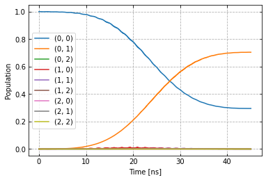
Dynamics

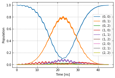
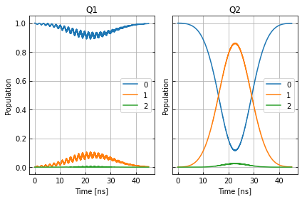
The system is initialised in the state \(|0,1\rangle\) so that a transition to \(|1,1\rangle\) should be visible.

psi_init = [[0] * 9]
psi_init[0][0] = 1
init_state = tf.transpose(tf.constant(psi_init, tf.complex128))
print(init_state)

tf.Tensor(
[[1.+0.j]
 [0.+0.j]
 [0.+0.j]
 [0.+0.j]
 [0.+0.j]
 [0.+0.j]
 [0.+0.j]
 [0.+0.j]
 [0.+0.j]], shape=(9, 1), dtype=complex128)

def plot_dynamics(exp, psi_init, seq):
        """
        Plotting code for time-resolved populations.

        Parameters
        ----------
        psi_init: tf.Tensor
            Initial state or density matrix.
        seq: list
            List of operations to apply to the initial state.
        """
        model = exp.pmap.model
        dUs = exp.partial_propagators
        psi_t = psi_init.numpy()
        pop_t = exp.populations(psi_t, model.lindbladian)
        for gate in seq:
            for du in dUs[gate]:
                psi_t = np.matmul(du.numpy(), psi_t)
                pops = exp.populations(psi_t, model.lindbladian)
                pop_t = np.append(pop_t, pops, axis=1)

        fig, axs = plt.subplots(1, 1)
        ts = exp.ts
        dt = ts[1] - ts[0]
        ts = np.linspace(0.0, dt*pop_t.shape[1], pop_t.shape[1])
        axs.plot(ts / 1e-9, pop_t.T)
        axs.grid(linestyle="--")
        axs.tick_params(
            direction="in", left=True, right=True, top=True, bottom=True
        )
        axs.set_xlabel('Time [ns]')
        axs.set_ylabel('Population')
        plt.legend(model.state_labels)
        pass

def getQubitsPopulation(population: np.array, dims: List[int]) -> np.array:
    """
    Splits the population of all levels of a system into the populations of levels per subsystem.
    Parameters
    ----------
    population: np.array
        The time dependent population of each energy level. First dimension: level index, second dimension: time.
    dims: List[int]
        The number of levels for each subsystem.
    Returns
    -------
    np.array
        The time-dependent population of energy levels for each subsystem. First dimension: subsystem index, second
        dimension: level index, third dimension: time.
    """
    numQubits = len(dims)

    # create a list of all levels
    qubit_levels = []
    for dim in dims:
        qubit_levels.append(list(range(dim)))
    combined_levels = list(itertools.product(*qubit_levels))

    # calculate populations
    qubitsPopulations = np.zeros((numQubits, dims[0], population.shape[1]))
    for idx, levels in enumerate(combined_levels):
        for i in range(numQubits):
            qubitsPopulations[i, levels[i]] += population[idx]
    return qubitsPopulations

def plotSplittedPopulation(
    exp: Exp,
    psi_init: tf.Tensor,
    sequence: List[str]
) -> None:
    """
    Plots time dependent populations for multiple qubits in separate plots.
    Parameters
    ----------
    exp: Experiment
        The experiment containing the model and propagators
    psi_init: np.array
        Initial state vector
    sequence: List[str]
        List of gate names that will be applied to the state
    -------
    """
    # calculate the time dependent level population
    model = exp.pmap.model
    dUs = exp.partial_propagators
    psi_t = psi_init.numpy()
    pop_t = exp.populations(psi_t, model.lindbladian)
    for gate in sequence:
        for du in dUs[gate]:
            psi_t = np.matmul(du, psi_t)
            pops = exp.populations(psi_t, model.lindbladian)
            pop_t = np.append(pop_t, pops, axis=1)
    dims = [s.hilbert_dim for s in model.subsystems.values()]
    splitted = getQubitsPopulation(pop_t, dims)

    # timestamps
    dt = exp.ts[1] - exp.ts[0]
    ts = np.linspace(0.0, dt * pop_t.shape[1], pop_t.shape[1])

    # create both subplots
    titles = list(exp.pmap.model.subsystems.keys())
    fig, axs = plt.subplots(1, len(splitted), sharey="all")
    for idx, ax in enumerate(axs):
        ax.plot(ts / 1e-9, splitted[idx].T)
        ax.tick_params(direction="in", left=True, right=True, top=False, bottom=True)
        ax.set_xlabel("Time [ns]")
        ax.set_ylabel("Population")
        ax.set_title(titles[idx])
        ax.legend([str(x) for x in np.arange(dims[idx])])
        ax.grid()

    plt.tight_layout()
    plt.show()

sequence = [cnot12.get_key()]
plot_dynamics(exp, init_state, sequence)
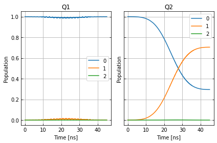
plotSplittedPopulation(exp, init_state, sequence)

Visualisation with qiskit circuit

qc = QuantumCircuit(2, 2)
qc.append(RX90pGate(), [0])
qc.cx(0, 1)
qc.draw()

     ┌────────────┐
q_0: ┤ Rx90p(π/2) ├──■──
     └────────────┘┌─┴─┐
q_1: ──────────────┤ X ├
                   └───┘
c: 2/═══════════════════
                        

c3_provider = C3Provider()
c3_backend = c3_provider.get_backend("c3_qasm_physics_simulator")
c3_backend.set_c3_experiment(exp)

c3_job_unopt = c3_backend.run(qc)
result_unopt = c3_job_unopt.result()
res_pops_unopt = result_unopt.data()["state_pops"]
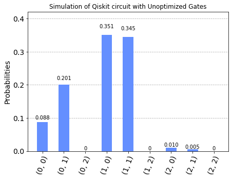
print("Result from unoptimized gates:")
pprint(res_pops_unopt)

No measurements in circuit "circuit-0", classical register will remain all zeros.

Result from unoptimized gates:
{'(0, 0)': 0.08793249061599799,
 '(0, 1)': 0.20140214999016118,
 '(0, 2)': 1.7916216253388795e-05,
 '(1, 0)': 0.3507070201094552,
 '(1, 1)': 0.34492529411056444,
 '(1, 2)': 5.054006496570894e-06,
 '(2, 0)': 0.009940433069486916,
 '(2, 1)': 0.005069321214083548,
 '(2, 2)': 3.20667334658816e-07}

plot_histogram(res_pops_unopt, title='Simulation of Qiskit circuit with Unoptimized Gates')

Open-loop optimal control

Now, open-loop optimisation with DRAG enabled is set up.

generator.devices['AWG'].enable_drag_2()

opt_gates = [cnot12.get_key()]
exp.set_opt_gates(opt_gates)

gateset_opt_map=[
    [(cnot12.get_key(), "d1", "gauss1", "amp")],
    [(cnot12.get_key(), "d1", "gauss1", "freq_offset")],
    [(cnot12.get_key(), "d1", "gauss1", "xy_angle")],
    [(cnot12.get_key(), "d1", "gauss1", "delta")],
    [(cnot12.get_key(), "d1", "carrier", "framechange")],
    [(cnot12.get_key(), "d2", "gauss2", "amp")],
    [(cnot12.get_key(), "d2", "gauss2", "freq_offset")],
    [(cnot12.get_key(), "d2", "gauss2", "xy_angle")],
    [(cnot12.get_key(), "d2", "gauss2", "delta")],
    [(cnot12.get_key(), "d2", "carrier", "framechange")],
]
parameter_map.set_opt_map(gateset_opt_map)

parameter_map.print_parameters()

cx[0, 1]-d1-gauss1-amp                : 800.000 mV
cx[0, 1]-d1-gauss1-freq_offset        : -53.000 MHz 2pi
cx[0, 1]-d1-gauss1-xy_angle           : -444.089 arad
cx[0, 1]-d1-gauss1-delta              : -1.000
cx[0, 1]-d1-carrier-framechange       : 4.712 rad
cx[0, 1]-d2-gauss2-amp                : 30.000 mV
cx[0, 1]-d2-gauss2-freq_offset        : -53.000 MHz 2pi
cx[0, 1]-d2-gauss2-xy_angle           : -444.089 arad
cx[0, 1]-d2-gauss2-delta              : -1.000
cx[0, 1]-d2-carrier-framechange       : 0.000 rad

As a fidelity function we choose unitary fidelity as well as LBFG-S (a wrapper of the scipy implementation) from our library.

import os
import tempfile
from c3.optimizers.optimalcontrol import OptimalControl

log_dir = os.path.join(tempfile.TemporaryDirectory().name, "c3logs")
opt = OptimalControl(
    dir_path=log_dir,
    fid_func=fidelities.unitary_infid_set,
    fid_subspace=["Q1", "Q2"],
    pmap=parameter_map,
    algorithm=algorithms.lbfgs,
    options={
        "maxfun": 25
    },
    run_name="cnot12"
)

Start the optimisation

exp.set_opt_gates(opt_gates)
opt.set_exp(exp)
opt.optimize_controls()

C3:STATUS:Saving as: /var/folders/04/np4lgk2d7sq6w0dpn758sgp80000gn/T/tmpryftkry4/c3logs/cnot12/2022_01_01_T_20_55_19/open_loop.c3log

The final parameters and the fidelity are

parameter_map.print_parameters()
print(opt.current_best_goal)

cx[0, 1]-d1-gauss1-amp                : 2.359 V
cx[0, 1]-d1-gauss1-freq_offset        : -53.252 MHz 2pi
cx[0, 1]-d1-gauss1-xy_angle           : 587.818 mrad
cx[0, 1]-d1-gauss1-delta              : -743.473 m
cx[0, 1]-d1-carrier-framechange       : -815.216 mrad
cx[0, 1]-d2-gauss2-amp                : 56.719 mV
cx[0, 1]-d2-gauss2-freq_offset        : -53.176 MHz 2pi
cx[0, 1]-d2-gauss2-xy_angle           : -135.515 mrad
cx[0, 1]-d2-gauss2-delta              : -519.864 m
cx[0, 1]-d2-carrier-framechange       : 598.919 mrad

0.0055213431696764514

Results of the optimisation

Plotting the dynamics with the same initial state:

plot_dynamics(exp, init_state, sequence)
plotSplittedPopulation(exp, init_state, sequence)

Now we plot the dynamics for the control in the excited state.

psi_init = [[0] * 9]
psi_init[0][4] = 1
init_state = tf.transpose(tf.constant(psi_init, tf.complex128))
print(init_state)

plot_dynamics(exp, init_state, sequence)
plotSplittedPopulation(exp, init_state, sequence)

tf.Tensor(
[[0.+0.j]
 [0.+0.j]
 [0.+0.j]
 [0.+0.j]
 [1.+0.j]
 [0.+0.j]
 [0.+0.j]
 [0.+0.j]
 [0.+0.j]], shape=(9, 1), dtype=complex128)

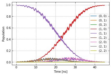
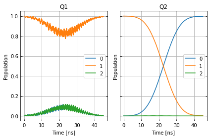
As intended, the dynamics of the target is dependent on the control qubit performing a flip if the control is excited and an identity otherwise.

Optimizing the single qubit gate on Qubit 1

opt_gates = [rx90p_q1.get_key()]
gateset_opt_map=[
    [
      (rx90p_q1.get_key(), "d1", "gauss", "amp"),
    ],
    [
      (rx90p_q1.get_key(), "d1", "gauss", "freq_offset"),
    ],
    [
      (rx90p_q1.get_key(), "d1", "gauss", "xy_angle"),
    ],
    [
      (rx90p_q1.get_key(), "d1", "gauss", "delta"),
    ],
    [
      (rx90p_q1.get_key(), "d1", "carrier", "framechange"),
    ]
]
parameter_map.set_opt_map(gateset_opt_map)
parameter_map.print_parameters()

rx90p[0]-d1-gauss-amp                 : 500.000 mV
rx90p[0]-d1-gauss-freq_offset         : -53.000 MHz 2pi
rx90p[0]-d1-gauss-xy_angle            : -444.089 arad
rx90p[0]-d1-gauss-delta               : -1.000
rx90p[0]-d1-carrier-framechange       : 0.000 rad

opt_1Q = OptimalControl(
    dir_path=log_dir,
    fid_func=fidelities.unitary_infid_set,
    fid_subspace=["Q1", "Q2"],
    pmap=parameter_map,
    algorithm=algorithms.lbfgs,
    options={
        "maxfun": 25
    },
    run_name="rx90p_q1"
)

exp.set_opt_gates(opt_gates)
opt_1Q.set_exp(exp)
opt_1Q.optimize_controls()

C3:STATUS:Saving as: /var/folders/04/np4lgk2d7sq6w0dpn758sgp80000gn/T/tmpryftkry4/c3logs/rx90p_q1/2022_01_01_T_20_58_09/open_loop.c3log

parameter_map.print_parameters()
print(opt_1Q.current_best_goal)

rx90p[0]-d1-gauss-amp                 : 390.140 mV
rx90p[0]-d1-gauss-freq_offset         : -52.986 MHz 2pi
rx90p[0]-d1-gauss-xy_angle            : -195.771 mrad
rx90p[0]-d1-gauss-delta               : -964.376 m
rx90p[0]-d1-carrier-framechange       : -282.109 mrad

0.00575481536619904

Before running the qiskit simulation, we must call set_opt_gates() to ensure propagators are calculated for all the required gates

exp.set_opt_gates([rx90p_q1.get_key(), cnot12.get_key()])

c3_job_opt = c3_backend.run(qc)
result_opt = c3_job_opt.result()
res_pops_opt = result_opt.data()["state_pops"]
print("Result from gates:")
pprint(res_pops_opt)

No measurements in circuit "circuit-0", classical register will remain all zeros.

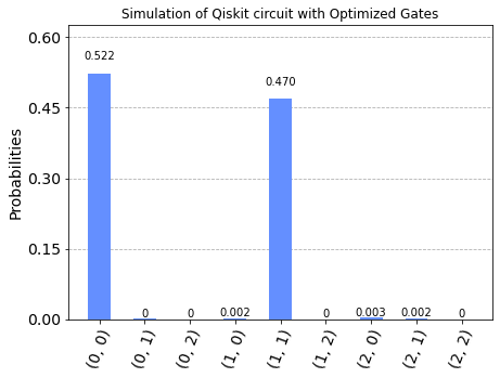
Result from gates:
{'(0, 0)': 0.522074672738806,
 '(0, 1)': 0.0009262330305873641,
 '(0, 2)': 5.58398828418534e-07,
 '(1, 0)': 0.002148790053836785,
 '(1, 1)': 0.4695772823691831,
 '(1, 2)': 3.241481428134574e-05,
 '(2, 0)': 0.0030096031488172107,
 '(2, 1)': 0.0022302669196215767,
 '(2, 2)': 1.7852604795947343e-07}

plot_histogram(res_pops_opt, title='Simulation of Qiskit circuit with Optimized Gates')